Introduction
With the continuous evolution of large language models (LLMs), researchers are exploring and pushing the boundaries of what these models can achieve. The demand for enhanced performance has increased with each new architecture and expanded parameter set, which is creating the necessity for advancement in LLM training methods.
The size and complexity of modern LLMs demand significant computational resources. This is where cloud-based GPUs are required. These cloud GPUs can execute multiple complex mathematical operations in parallel, which makes them very fast and efficient.
But apart from computational resources, latency and accuracy emerge as important factors affecting the performance of LLMs. The demand for fast, accurate model responses has increased, which motivates researchers to explore new and different training methods for LLMs.
Let’s dive deeper into this subject.
Overview of LLM Training Methods
There are three main methods to train large language models. Let’s look at them one by one.
-
Unsupervised Pre-training: This is the initial phase of training which focuses on exposing the model to a vast amount of text data. The input quantity is high, but the quality of the response is low. In this phase, the model is trained to predict the next probable token for a trillion sequence of texts. The output of this phase generally gives the foundation or base model.
-
Supervised Fine-Tuning: After the unsupervised pre-training, the model goes under supervised finetuning which is aimed at tailoring its capabilities to specific tasks or domains. In this phase, the model is provided with a smaller but high-quality dataset which consists of pairs of prompts and corresponding responses. By training on this dataset, the model learns to generate responses in line with the given prompts, which effectively transforms the base model into a specialized tool. This step is often referred to as ‘instruction tuning’, as it involves the fine-tuning of the model based on the explicit instructions provided by the training data.
-
Reinforcement Learning from Human Feedback (RLHF): This is the final phase which introduces reinforcement learning techniques. It leverages human feedback to further refine the model’s performance. This process unfolds in two stages:
-
Training a Reward Model: Initially, a reward model is trained to serve as a scoring function that assesses the quality of the generated responses. Human labelers evaluate responses and provide feedback, which is used to train the reward model.
-
Optimizing the LLM: After the reward model training, the LLM undergoes iterative optimization to generate responses that elicit high scores from the reward model. This optimization process involves adjusting the model's parameters to enhance the quality of the generated text while it adheres to constraints such as maintaining consistency and avoiding deterioration in performance. Essentially, the goal is to learn an optimal strategy or policy, for generating text that aligns with human preferences and constraints.
This final phase requires careful orchestration; it involves balancing the pursuit of higher-quality outputs with the need to maintain coherence and effectiveness in text completion. Through a combination of sophisticated algorithms and human-guided feedback, the LLM evolves into a powerful tool that is capable of producing contextually relevant and coherent text across various applications and domains.
Accelerating with E2E Cloud GPUs
In the context of the outlined LLM training process, cloud GPUs play an important role in accelerating the computational tasks involved in each stage. During the unsupervised pre-training phase, the LLM is exposed to massive amounts of data, and it requires extensive computational resources to process and analyze this data efficiently. Cloud GPUs excel in parallel computing, which enables the model to train on vast datasets in a fraction of the time it would take with traditional CPUs. The parallel processing capabilities of GPUs allow for simultaneous computation of multiple operations, which significantly speeds up the training process and reduces time to completion.
In the supervised fine-tuning stage, the model is further refined based on specific tasks or domains, which necessitates iterative training on high-quality datasets. Cloud GPUs enable fast experimentation and iteration by providing scalable computing resources on demand. Researchers and developers can quickly deploy GPU instances in the cloud, which allows them to train and evaluate different versions of the model in parallel, by accelerating the optimization process and facilitating faster convergence to optimal performance.
In the RLHF phase, the iterative optimization process relies heavily on computational resources to train the reward model and optimize the LLM based on human feedback. Cloud GPUs enable researchers and developers to scale up the training of complex reinforcement learning algorithms, such as policy gradient methods, which require extensive computational power for training neural networks. By harnessing the parallel processing capabilities of cloud GPUs, researchers and developers can accelerate the training of the reward model and expedite the optimization of the LLM, which leads to more efficient learning and improved performance.
E2E Networks provides a variety of advanced cloud GPUs that can accelerate the LLM training process. For more information about the products of E2E Networks, visit here.
To get started with E2E Cloud GPUs, login into your E2E account. Set up your SSH keys by visiting Settings.

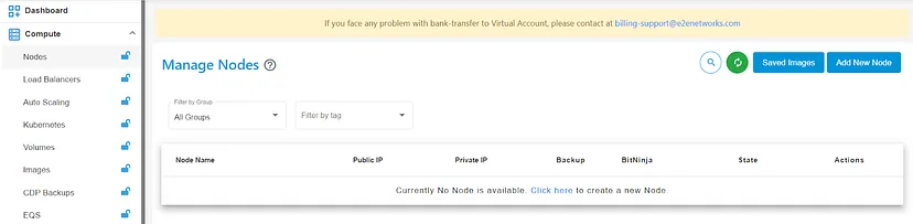
After creating the SSH keys, visit Compute to create a node instance.
Open your Visual Studio code, and download the extension Remote Explorer and Remote SSH. Open a new terminal. Login into your local system with the following code:
ssh root@
With this, you’ll be logged in to your node.
To see the performance of a model with different training methods, here we are using the Llama 2 model.
A Brief Introduction to Llama 2
Llama 2 represents a significant advancement in large language models; it was introduced by Meta AI in 2023 to democratize access to powerful AI capabilities for both research and commercial endeavors. Llama 2 is offered free of charge and is designed to excel in various natural language processing tasks, from text generation to programming code comprehension.
Unlike its predecessor, Llama 1, which was initially accessible only to select research institutions under specific licensing conditions, Llama 2 is available to any organization with fewer than 700 million active users. Llama 2 adopts a strategy of prioritizing model performance enhancement over sheer parameter count, which enables smaller organizations and research communities to leverage its capabilities without exorbitant computational costs by featuring models with varying parameters.
Llama 2 comprises a series of transformer-based autoregressive causal language models. These models operate by taking a sequence of words as input and recursively predicting the next word. During self-supervised pre-training, LLMs are fed the beginnings of sample sentences drawn from an extensive corpus of unlabeled data. Their task is to predict the subsequent word, training the model to minimize the discrepancy between the actual next word and its own predictions. Base foundation models are fundamentally not pre-trained to directly respond to prompts; instead, they append text to prompts in a grammatically coherent manner. Further refinement can be achieved through techniques like supervised learning and reinforcement learning, which is necessary to tailor a foundation model for specific applications such as dialogue systems, instruction following, or creative writing. Llama 2 models serve as a foundational framework for building purpose-specific models.
Unsupervised Pre-training with Base Model Llama 2
Let’s see how a foundation model under unsupervised pre-training goes with the Llama 2 model.
To get started, load the model.
from transformers import (
    AutoModelForCausalLM,
    AutoTokenizer,
    BitsAndBytesConfig,
    TrainingArguments,
    pipeline,
    logging,
)
from peft import LoraConfig
from trl import SFTTrainer

model = AutoModelForCausalLM.from_pretrained("NousResearch/Llama-2-7b-chat-hf", device_map="auto")
There is one flag while loading the model, i.e., device_map. It ensures that the model is moved to your GPU.
Then, we will load the tokenizer with the same model that we loaded before.
import torch
tokenizer = AutoTokenizer.from_pretrained("NousResearch/Llama-2-7b-chat-hf", padding_side="left")
Tokenizer.pad_token = tokenizer.eos_token
Now, we’ll preprocess the text input with the tokenizer. The model_inputs variable holds the tokenized text input as well as the attention masks. After tokenizing the inputs, the generate method will return the generated tokens.
model_inputs = tokenizer(["India is", "The future of AI is"], return_tensors="pt", padding=True).to("cuda")
generated_ids = model.generate(**model_inputs,max_new_tokens=50)
tokenizer.batch_decode(generated_ids, skip_special_tokens=True)
The following will be the result:
['India is a country with a diverse culture and a long history. It is home to many different ethnic groups, each with their own unique traditions and customs. In this essay, we will explore some of the main ethnic groups in India and',
 'The future of AI is exciting and uncertain\n\nThe future of AI is exciting and uncertain. On one hand, AI has the potential to revolutionize numerous industries and aspects of society, from healthcare and education to transportation and entertainment. On']
As the maximum number of new tokens is 50, it has generated text according to that.
Supervised Fine-Tuning with Llama 2
As we noticed, the unsupervised pre-trained model is performing well, but to train the particular model on a specific dataset, so that it could generate responses accordingly, we will move to supervised fine-tuning.
To get started, we will first load the dataset. I have picked a Llama dataset from Hugging Face, which can be found here.
from datasets import load_dataset
dataset = load_dataset("mlabonne/guanaco-llama2-1k", split="train")
Now, we will use 4-bit quantization and set the quantization configuration to the model to improve the speed.
bnb_4bit_compute_dtype = "float16"
compute_dtype = getattr(torch, bnb_4bit_compute_dtype)

bnb_config = BitsAndBytesConfig(
   load_in_4bit=True,
   bnb_4bit_quant_type="nf4",
   bnb_4bit_compute_dtype=compute_dtype,
   bnb_4bit_use_double_quant=False,
)
Now, load the model.
model = AutoModelForCausalLM.from_pretrained(
    "NousResearch/Llama-2-7b-chat-hf",
    quantization_config=bnb_config,
    device_map={"": 0},
    trust_remote_code=True,
    num_labels=1,
)
model.config.use_cache = False
Load the tokenizer and set the padding side to the right to overcome the issues with FP16.
tokenizer = AutoTokenizer.from_pretrained("NousResearch/Llama-2-7b-chat-hf", trust_remote_code=True)
tokenizer.pad_token = tokenizer.eos_token
tokenizer.padding_side = "right"
Now, define the PEFT parameters. We’ll be using LoRA and setting the configurations according to that.
peft_params = LoraConfig(
    lora_alpha=16,
    lora_dropout=0.1,
    r=64,
    bias="none",
    task_type="CAUSAL_LM",
)
Then, we’ll define the training parameters. But, before that, we’ll make a directory to store the output.
%mkdir /root/results
The training results can be reported to the TensorBoard or Weights & Biases, but I have used TensorBoard here. Before passing the TrainingArguments, make sure that TensorFlow and TensorBoard are installed in your node.
The training parameters will look like this:
training_args = TrainingArguments(
    output_dir="/root/results",
    max_steps=300,
    per_device_train_batch_size=4,
    gradient_accumulation_steps=1,
    learning_rate=1.4e-5,
    optim="adamw_torch",
    save_steps=50,
    logging_steps=50,
    report_to="tensorboard",
    remove_unused_columns=False,
)
Now to fine-tune the model under supervised training, we’ll pass the model, training dataset, tokenizer, PEFT configurations, dataset text field, maximum sequence length, and training parameters to the SFT trainer, which is a module under the TRL library. TRL library is a Hugging Face library, especially for reinforcement learning.
trainer = SFTTrainer(
    model=model,
    train_dataset=dataset,
    peft_config=peft_params,
    dataset_text_field="text",
    max_seq_length=None,
    tokenizer=tokenizer,
    args=training_args,
    packing=False,
)
Then, we’ll train the model and save the model.
trainer.train()
trainer.model.save_pretrained("root/model/sft_model")
Using the text generation pipeline, we’ll pass the prompt and get the responses accordingly.
pipe = pipeline(task="text-generation", model=model, tokenizer=tokenizer, max_length=200)
Reinforcement Learning from Human Feedback
To refine the model’s performance and assess the quality of the response, we move to the RLHF training.
First, we’ll train a reward model and then optimize the LLM.
Reward Modeling
To create a reward model, you can create a reward model class, or simply use the RewardTrainer from TRL Hugging Face library.
Reward model class can be defined as:
class RewardTrainer(Trainer):
    def compute_loss(self, model, inputs, return_outputs=False):
        # Compute rewards for inputs 'j' and 'k' using the provided model
        rewards_j = model(input_ids=inputs["input_ids_j"], attention_mask=inputs["attention_mask_j"])[0]
        rewards_k = model(input_ids=inputs["input_ids_k"], attention_mask=inputs["attention_mask_k"])[0]
        # Compute the negative log-sigmoid loss between the rewards
        loss = -nn.functional.logsigmoid(rewards_j - rewards_k).mean()
        if return_outputs:
            # Return loss and rewards for debugging or monitoring purposes
            return loss, {"rewards_j": rewards_j, "rewards_k": rewards_k}
        return loss
If you’re choosing to use RewardTrainer, then it expects a very specific format for the dataset. It uses four entries, which are:
- input_ids_chosen
- attention_mask_chosen
- input_ids_rejected
- attention_mask_rejected
For reward modeling, I have used this dataset, which meets the requirements of RewardTrainer already.
train_dataset = load_dataset("Anthropic/hh-rlhf", split="train")
Then, we’ll define the preprocessing function in which all four entries will be there.
def preprocess_function(examples):
    new_examples = {
        "input_ids_chosen": [],
        "attention_mask_chosen": [],
        "input_ids_rejected": [],
        "attention_mask_rejected": [],
    }
    for chosen, rejected in zip(examples["chosen"], examples["rejected"]):
        tokenized_j = tokenizer(chosen, truncation=True)
        tokenized_k = tokenizer(rejected, truncation=True)

       new_examples["input_ids_chosen"].append(tokenized_j["input_ids"])
        new_examples["attention_mask_chosen"].append(tokenized_j["attention_mask"])
        new_examples["input_ids_rejected"].append(tokenized_k["input_ids"])
        new_examples["attention_mask_rejected"].append(tokenized_k["attention_mask"])

   return new_examples
We’ll map the dataset to the preprocessing function in batches.
# Apply preprocess_function to the training dataset in parallel using multiple processes

train_dataset = train_dataset.map(
    preprocess_function,
    batched=True,
    num_proc=4,
)

# Filter the dataset to remove examples where the length of input_ids_chosen and input_ids_rejected exceeds 512 tokens

train_dataset = train_dataset.filter(
    lambda x: len(x["input_ids_chosen"]) <= 512=""  =""  and="" len(x["input_ids_rejected"])="" <="512" )="" code="">
Then, we’ll pass the quantized model, tokenizer, training arguments, dataset, and PEFTconfiguration to the RewardTrainer.
trainer = RewardTrainer(
    model=model,
    tokenizer=tokenizer,
    args=training_args,
    train_dataset=train_dataset,
    peft_config=peft_params,
    max_length=512,
)
After that, we’ll train and save the model.
trainer.train()
trainer.model.save_pretrained("root/model/reward_model")
LLM Optimization
There are many optimization techniques to optimize an LLM, but Direct Preference Optimization and Proximal Policy Optimization are mostly used with the reward model. DPO is used when the reward function is not defined, while PPO works with the reward function. Here, we defined the Reward function using RewardTrainer.
Proximal Policy Optimization
The PPOTrainer has the requirement to align a generated response with a query where the rewards are obtained from the reward model. In each step of the PPO Trainer, a batch of prompts is sampled from the dataset, and then these prompts are used to generate the responses from the SFT model.
After that, the reward model is used to compute the rewards for the generated response. At last, these computed rewards are used to optimize the SFT model using the PPO Trainer.
PPO trainer expects the dataset to have the text column so that it can be renamed to query later. In the Reward training model, we used this dataset, where the columns are ‘chosen’ and ‘rejected’. But here in PPO training, we have to select one column which we can rename to ‘query’, which is a PPO trainer’s requirement.
train_dataset = train_dataset.rename_column("chosen", "query")
train_dataset = train_dataset.remove_columns(["rejected"])
Now, initialize the PPO trainer by setting its configuration.
from trl import PPOConfig
config = PPOConfig(
    model_name="NousResearch/Llama-2-7b-chat-hf",
    learning_rate=1.4e-5,
)
After that, we will initialize our model. PPO requires a reference model which is generated by the PPOTrainer automatically.
from trl import AutoModelForCausalLMWithValueHead, PPOConfig, PPOTrainer

model = AutoModelForCausalLMWithValueHead.from_pretrained(config.model_name)
tokenizer = AutoTokenizer.from_pretrained(config.model_name)

tokenizer.pad_token = tokenizer.eos_token
Then we will train the PPO trainer with the SFT model, PPO configurations, dataset, and tokenizer. After that, we’ll save the model.
from trl import PPOTrainer

ppo_trainer = PPOTrainer(
    model=model,
    config=config,
    train_dataset=train_dataset,
    tokenizer=tokenizer,
)
ppo_trainer.train()
ppo_trainer.model.save_pretrained("root/model/ppo_model")
Direct Preference Optimization
The DPO trainer also expects a very specific format for the dataset. Using the DPO trainer, the model will be trained to directly optimize preference for the sentence that is most relevant, given two sentences.
The DPO trainer requires these three entries:
- Prompt
- Chosen
- Rejected
In our dataset, chosen and rejected are already present, but the prompt column is not there. Just for an experiment, I generated the relevant prompt manually and added the prompt column to the dataset.
def generate_prompt(chosen_text, rejected_text):
    # Combine the chosen and rejected text to form a prompt
    prompt = f"Given the chosen text: '{chosen_text}', and the rejected text: '{rejected_text}', please provide a response."
    return prompt

for example in train_dataset:
    # Generate prompt based on 'chosen' and 'rejected' columns
    prompt = generate_prompt(example['chosen'], example['rejected'])
    # Add the generated prompt to the dataset
    example['prompt'] = prompt
After this, my dataset meets the expectation of a DPO Trainer. We’ll initialize the DPO Trainer by passing the SFT model, training arguments, dataset, and tokenizer. We’ll train the model with a DPO trainer and save the model.
dpo_trainer = DPOTrainer(
    model,
    model_ref=None,
    args=training_args,
    beta=0.1,
    train_dataset=train_dataset,
    tokenizer=tokenizer,
)
dpo_trainer.train()
dpo_trainer.model.save_pretrained("root/model/dpo_model")
Conclusion
From unsupervised pretrained models to optimized models using reinforcement learning, we have explored various training methods for large language models. We utilized E2E Network’s Cloud GPUs to train different models for efficacy and efficient performance. Since all the models are saved in your directory, it’s your time to experiment with them and monitor their responses with respect to your datasets.
Thanks for reading!