
Large language models generate text one token at a time. For each token, the model runs a complete forward pass through billions of parameters, produces the next word, then repeats the entire process for the following token. This sequential nature is the bottleneck. You can't predict the fifth token until you've generated the fourth, which means the GPU spends most of its time waiting on memory transfers rather than doing actual computation. This sequential bottleneck is why faster LLM inference has become critical for production deployments.
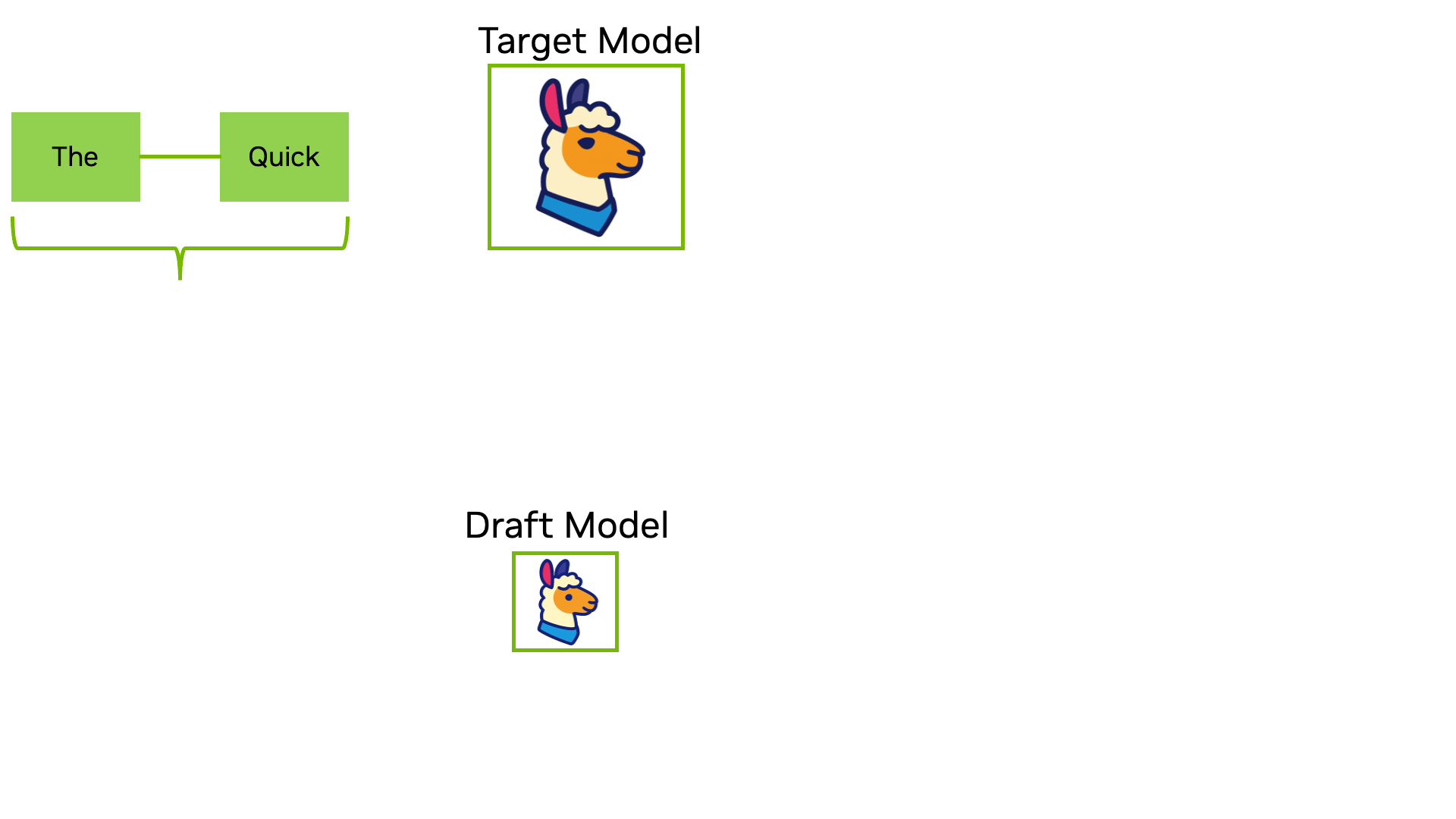
Speculative decoding breaks this pattern. Instead of generating one token at a time, you use a small draft model to predict several tokens ahead, then verify all of them at once with the main model. When the draft model's predictions are good, you get 4-6 tokens from a single verification pass instead of running the main model 4-6 times. The main model still makes the final decision on every token, so the output quality is identical to standard generation, you're just doing the work in parallel instead of sequentially.
Traditional speculative decoding approaches use a separate, smaller model as the draft model typically from the same model family, like using Llama-8B to accelerate Llama-70B. This creates challenges around model availability, training costs, and ensuring the draft model matches the target model's distribution.
EAGLE-3 takes a different approach. Instead of using a completely separate model, it trains a lightweight draft head that plugs into the target model and reuses its internal features. This draft head is much smaller than a full model, just 1-2 transformer layers instead of dozens. The key innovation in EAGLE-3 is how this draft head is trained. Through a technique called training-time testing, EAGLE-3 simulates the actual inference conditions during training, which addresses the distribution mismatch problem that hurts traditional methods. It also fuses information from multiple layers of the target model instead of relying only on the top layer.
The approach delivers speedups between 3x to 6.5x compared to standard autoregressive generation, with better scaling behavior when you add more training data.
This post walks through how EAGLE-3 works, why it outperforms earlier methods, and how to implement it for your own models.
What is Speculative Decoding?
Speculative decoding is an LLM inference optimization technique that generates multiple tokens in parallel instead of one at a time. A small draft model predicts several candidate tokens ahead, which are then verified simultaneously by the main model in a single forward pass. This approach achieves 2-6x faster inference while maintaining identical output quality to standard autoregressive generation.
The Problem with Traditional Speculative Decoding
Traditional speculative decoding relies on a two-model system. You run a smaller draft model that quickly generates several candidate tokens, then feed those candidates to the larger target model for verification. The target model processes all candidates in a single forward pass and decides which ones to keep. If the draft model's predictions are good, you accept multiple tokens at once. If they're wrong, you discard them and continue from the last good token.
 Traditional speculative decoding workflow: A draft model generates candidate tokens, which are then verified in parallel by the target model. (Source: NVIDIA Developer Blog)
The draft model is typically a smaller version from the same model family. If you're accelerating Llama-70B, you might use Llama-8B as your draft model. For Qwen2-72B, you'd use Qwen2-7B. This requirement creates several practical challenges.
Get ₹2,000 free credits to test your AI workloads
Sign up and complete ID verification to unlock free credits. Deploy on NVIDIA H200, H100, and L40S GPUs—no commitment required.
The Tokenizer Compatibility Constraint
Traditional speculative decoding has a hard requirement: the draft and target models must share the same tokenizer and vocabulary. The verification step compares probability distributions from both models for the same token IDs.
In practice, the easiest way to ensure tokenizer compatibility is to use a smaller model from the same family as your target model. Llama-3.1-8B as a draft for Llama-3.1-70B works because they share the exact same tokenizer and vocabulary. Same family also means similar training data and output distributions, which improves acceptance rates. You could technically use draft models from different architectures as long as they share the tokenizer, but acceptance rates drop when the models learned different patterns.
The problem shows up when your target model doesn't have a smaller sibling with the same tokenizer. Many production models ship as single sizes without a corresponding model family. If you have a capable 70B model but no compatible 7B or 13B version, you'd need to train your own draft model from scratch or use techniques like EAGLE-style draft heads that avoid a separate full model altogether.
Training and Data Requirements
Even when a smaller model exists in the same family, it might not be ideal for your use case. The draft model's acceptance rate is highest when its output distribution closely matches the target's. If you've fine-tuned your target model on domain-specific data, a vanilla base model from the same family can produce noticeably different outputs, which reduces acceptance rates and overall speedup.
For proprietary or privately trained models, you don't have access to the original training data, so it's harder to train a perfectly aligned draft model. Providers can ship a smaller sibling model or a built-in draft mechanism, but that adds engineering and release complexity on their side.
Get ₹2,000 free credits to test your AI workloads
Sign up and complete ID verification to unlock free credits. Deploy on NVIDIA H200, H100, and L40S GPUs—no commitment required.
The Independence Problem
In traditional two-model speculative decoding, the draft model operates completely independently from the target model. It doesn't use any information from the target model during inference. The draft model generates its predictions based solely on its own weights and training, then passes those predictions to the target model for verification.
This independence means the draft model has to learn everything on its own. The target and draft both process the same prefix, but they do so in separate networks. The draft doesn't get to reuse the target's intermediate representations—it must maintain its own full stack of layers to produce logits.
Why EAGLE Takes a Different Approach
The EAGLE family of methods addresses these problems by changing how the draft model works. Instead of using a completely separate independent model, EAGLE trains a lightweight draft head that attaches directly to the target model and reuses its internal features. This is still training, but you're training a small module (1-2 transformer layers) rather than an entire model.
EAGLE-3 pushes this further by improving how that draft head is trained and what information it uses from the target model. The result is a system that's more flexible, scales better with training data, and achieves higher acceptance rates.
EAGLE-3 Architecture: Advanced Speculative Decoding Design
Core Design Philosophy
EAGLE-3 abandons the idea that you need a separate draft model to accelerate inference. Instead of training a standalone draft model from scratch or relying on a smaller version from the same model family, EAGLE-3 trains a lightweight draft head that plugs directly into your target model.
The draft head is remarkably small: its core is a single Transformer decoder layer plus a few projection layers for fusing low/mid/high-level features and combining them with token embeddings. For a model like LLaMA-3.1-8B with 32 decoder layers, this is minimal overhead. The draft head adds well under 5% extra parameters even for 70B-scale models. This approach significantly reduces LLM inference cost by minimizing expensive forward passes through the target model. During training, it learns to predict tokens by fusing features from multiple layers of the target model, not just the top layer. Once trained, the same draft head works across different tasks (code generation, math reasoning, instruction following, summarization) without any task-specific fine-tuning, as demonstrated in the paper's experiments on MT-bench, HumanEval, GSM8K, Alpaca, and CNN/Daily Mail.
The key innovation is training-time test. When EAGLE-3 generates text during inference, it predicts multiple tokens ahead in sequence: after the first prediction, later predictions must rely on previous draft outputs instead of perfect target-model features. This creates a gap, because models are usually trained only on clean, ground-truth inputs but evaluated on their own noisy predictions.
EAGLE-3 closes this gap by simulating the actual generation process during training. Some positions see fused features from the target model, while others see the draft model's own outputs fed back in. This mixed regime matches what happens at inference. In the paper's MT-bench experiments, this lets EAGLE-3 keep a high, almost flat acceptance rate of around 70-80% across positions, whereas EAGLE's acceptance rate drops noticeably as more draft tokens appear in the context.
Now, let's dive into each layer of Eagle-3.
Multi-Layer Feature Fusion
The problem with top-layer-only approaches
Earlier EAGLE-style speculative methods like EAGLE and EAGLE-2 only use the top-layer features from the target model, the features right before the language modeling head. This makes sense because these features directly correspond to the next token's logits. But there's a catch: top-layer features are optimized for predicting the immediate next token. When you need to predict the token after that, or the token after that, you're asking these features to do something they weren't designed for.
EAGLE-3's solution: Multi-layer fusion
The information needed to predict multiple steps ahead exists in the model, but it's distributed across different layers. EAGLE-3 extracts features from three levels: low, middle, and high. Each level of the model captures different aspects of the input, and combining them gives the draft head richer information for multi-step prediction.
 Training architecture: The target model generates embeddings and hidden states at low, mid, and high layers. These features are concatenated and passed through an FC layer to produce fused hidden states, which feed into the draft model's decoder layer for plogp loss calculation. (Source: LMSYS SpecForge Blog)
Here's how the fusion works. For example, for a model like Llama-3.1-8B with hidden dimension 4096, each level produces a 4096-dimensional vector. EAGLE-3 concatenates these three vectors into a 12,288-dimensional vector, then compresses it back down to 4096 dimensions through a fully connected layer. This compression step learns which features from each level matter most for predicting multiple tokens ahead.
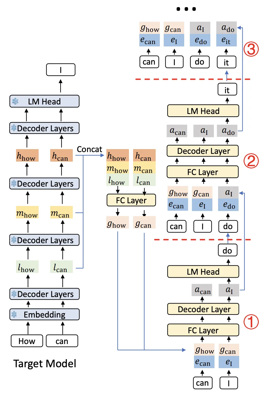 Complete inference workflow: The target model processes input tokens through multiple decoder layers. For each prompt position, features from low/mid/high layers are extracted, fused, and fed to the draft model's decoder. The draft model then generates a tree of candidate tokens (shown as nodes ①②③), which are verified by the target model's LM head in parallel. (Source: LMSYS SpecForge Blog)
When you generate text with the prompt "How can", the target model runs a forward pass and produces features at each layer. EAGLE-3 grabs features from all three levels, fuses them, and creates a unified representation that's useful for predicting not just "I" but also what comes after it.
The Draft Head Architecture
The draft head is remarkably simple - it's just one transformer decoder layer. That's it. Your typical target model has 28-32 layers, so this is minimal overhead.
How it works during inference:
When generating text, the draft head takes two inputs: the fused features from the target model and the embedding of the previously sampled token. These get concatenated and passed through an FC layer to reduce back to the hidden dimension. This goes into the single decoder layer, which produces an output. That output feeds into the target model's LM head to get the probability distribution over tokens, and then a token is sampled.
The draft head is a standard Transformer decoder block with the same hidden size and attention layout as the target model. The only part that needs modification is the self-attention component, which has to handle tree-like dependencies during training when the model trains on its own predictions.
The draft head adds only a small fraction of extra parameters (around 1-2% of the base model for Llama-3.1-8B and Llama-3.1-70B), so the memory overhead is modest compared to the target model itself. The computational overhead is minimal, one decoder layer versus the dozens in the target model. This lightweight design means you get significant speedups without meaningful memory or compute costs.
Tree-Based Generation and Verification
Vanilla autoregressive decoding generates one token at a time: pick the next token, generate it, then pick the next one. If your first guess is wrong, everything after it has to be recomputed. EAGLE-3 avoids this waste by generating a tree of candidates instead of a single sequence.
Step 1: Building the candidate tree
Start with the prompt "The weather is". The target model has just generated this prefix and produced features from its layers. The draft head takes these features and generates multiple candidates for the next token, the top-k options where k is configurable (for example, 4 or 8 via speculative-eagle-topk in SGLang).
Let's say it picks three: "sunny" (p=0.5), "getting" (p=0.3), and "very" (p=0.15). Now from each of these, the draft head generates continuations. From "sunny" it predicts "today" and "and". From "getting" it predicts "better" and "worse". From "very" it predicts "hot".
The result is a tree:
                The weather is
                      │
        ┌─────────────┼─────────────┐
        │             │             │
     sunny         getting        very
    (p=0.5)       (p=0.3)       (p=0.15)
        │             │             │
    ┌───┴───┐     ┌───┴───┐       hot
    │       │     │       │     (p=0.8)
  today    and  better  worse
 (p=0.7) (p=0.2)(p=0.6)(p=0.3)
This tree has 8 candidate tokens total: 3 at the first level and 5 at the second level.
Managing exponential growth
Without constraints, the tree would explode. With k=8 candidates per position and depth=5 levels, you'd get up to 8^5 = 32,768 possible leaf nodes. The draft model would spend all its time generating candidates, and the target model would be overwhelmed verifying thousands of tokens.
EAGLE-3 inherits the dynamic draft tree mechanism from EAGLE-2, which uses two controls to keep tree size manageable:
-
Confidence-based pruning during tree construction. When the draft head's confidence (softmax probability) drops below a threshold, that branch stops growing immediately. Low-probability branches get cut early before they spawn more descendants.
-
A fixed token budget for verification. After the tree is built, the implementation selects only the top N draft tokens to send to the target model (configured via
speculative-num-draft-tokensin SGLang). Candidates are ranked during a pruning stage, and only the best ones within the token budget get verified. Open-source configs typically use token budgets in the single to low double digits.
The result is adaptive. In predictable contexts like "The capital of France is", the tree extends deep along a single high-confidence path. In uncertain contexts like creative writing, it stays shallow with more branching. But the verification step always stays within the token budget.
Step 2: Verification with tree attention
The target model now needs to verify the selected candidates in one forward pass. But there's a constraint: each branch is a different timeline. Going back to our previous example, the token "today" in the "sunny → today" path shouldn't see "getting" or "worse" from other branches. Those tokens don't exist in its timeline.
Tree attention solves this with specialized attention masks. Each token only attends to its ancestors:
- "today" sees: ["The", "weather", "is", "sunny"]
- "better" sees: ["The", "weather", "is", "getting"]
- "hot" sees: ["The", "weather", "is", "very"]
Here's what the attention mask looks like for our weather tree:
| Query \ Keys | The | weather | is | sunny | getting | very | today | and | better | worse | hot |
|---|---|---|---|---|---|---|---|---|---|---|---|
| The | 1 | 0 | 0 | 0 | 0 | 0 | 0 | 0 | 0 | 0 | 0 |
| weather | 1 | 1 | 0 | 0 | 0 | 0 | 0 | 0 | 0 | 0 | 0 |
| is | 1 | 1 | 1 | 0 | 0 | 0 | 0 | 0 | 0 | 0 | 0 |
| sunny | 1 | 1 | 1 | 1 | 0 | 0 | 0 | 0 | 0 | 0 | 0 |
| getting | 1 | 1 | 1 | 0 | 1 | 0 | 0 | 0 | 0 | 0 | 0 |
| very | 1 | 1 | 1 | 0 | 0 | 1 | 0 | 0 | 0 | 0 | 0 |
| today | 1 | 1 | 1 | 1 | 0 | 0 | 1 | 0 | 0 | 0 | 0 |
| and | 1 | 1 | 1 | 1 | 0 | 0 | 0 | 1 | 0 | 0 | 0 |
| better | 1 | 1 | 1 | 0 | 1 | 0 | 0 | 0 | 1 | 0 | 0 |
| worse | 1 | 1 | 1 | 0 | 1 | 0 | 0 | 0 | 0 | 1 | 0 |
| hot | 1 | 1 | 1 | 0 | 0 | 1 | 0 | 0 | 0 | 0 | 1 |
Notice how "today" and "and" can both see "sunny" (their parent) but not "getting" or "very" (other branches). Similarly, "better" and "worse" see "getting" but not "sunny". This keeps each branch independent during verification.
The target model processes all candidates in parallel, producing probability distributions for each position. For a tree with N draft tokens, you get N probability distributions from one forward pass. This is where the speedup comes from: one forward pass verifies dozens of candidates instead of checking them one at a time.
Step 3: Acceptance using rejection sampling
The target model walks through the tree from the root, comparing its predictions against each draft token. For each candidate, it computes an acceptance probability: min(1, p_target/p_draft). If this equals 1.0, the token is automatically accepted. If it's less than 1.0, a random draw determines acceptance. Once a token is rejected, that entire branch and all its descendants are discarded.
To build intuition, let's walk through our weather example. If we look at a single candidate and imagine the case where p_target ≥ p_draft, the acceptance probability becomes 1 and the token is always accepted:
Check "sunny":
  p_draft("sunny") = 0.5
  p_target("sunny") = 0.6
  Since 0.6 > 0.5 → ✓ ACCEPTED

Check "today" (child of "sunny"):
  p_draft("today") = 0.7
  p_target("today") = 0.2
  Since 0.2 < 0.7 → ✗ REJECTED
  (This branch stops here)

Check "and" (child of "sunny"):
  p_draft("and") = 0.2
  p_target("and") = 0.8
  Since 0.8 > 0.2 → ✓ ACCEPTED

Check "getting" (sibling of "sunny"):
  p_draft("getting") = 0.3
  p_target("getting") = 0.1
  Since 0.1 < 0.3 → ✗ REJECTED
  (All descendants "better" and "worse" are discarded)

Check "very" (sibling of "sunny"):
  p_draft("very") = 0.15
  p_target("very") = 0.05
  Since 0.05 < 0.15 → ✗ REJECTED
  ("hot" is discarded)
The accepted path is "sunny → and". The target model then generates one additional token from "The weather is sunny and", and the drafting process starts over from this new prefix.
Why this works
The tree structure is dynamic and context-aware. It allocates more draft tokens where they're likely to succeed and fewer where prediction is hard. In predictable contexts, the tree extends deep along high-confidence paths. In uncertain contexts, it stays shallow with more branching. But the pruning mechanisms ensure the verification step stays within a manageable token budget.
The EAGLE-3 paper reports average acceptance lengths between 4.0 and 7.5 tokens depending on model and task. Those accepted tokens come from a single target model forward pass verifying the entire candidate tree, instead of running separate passes for each token. That's where the speedup comes from.
Training-Time Test: Solving Distribution Mismatch
The problem with traditional training
During inference, the draft head predicts multiple tokens ahead in sequence. The first predicted token uses perfect features from the target model. But the second predicted token has to use the first prediction as input. The third uses both previous predictions. And so on.
This creates a distribution mismatch. During training, traditional methods learn to predict the next token given perfect ground-truth features from the target model. But during inference, the draft head must work with its own imperfect predictions as inputs. For the first prediction, the inputs are perfect. For the second prediction, one input is the draft head's own output. For the fifth prediction, four inputs are the draft head's own outputs.
This mismatch causes acceptance rates to degrade over multiple steps. In EAGLE (without training-time test), the acceptance rate drops noticeably as more self-predicted inputs are used. The draft head trained on perfect inputs doesn't know how to handle its own noisy outputs.
Training-time test: Simulating inference during training
EAGLE-3 solves this by simulating the actual inference process during training. Instead of always training on perfect features, it trains on a mix: perfect features from the target model for early positions, and the draft head's own predictions for recent positions.
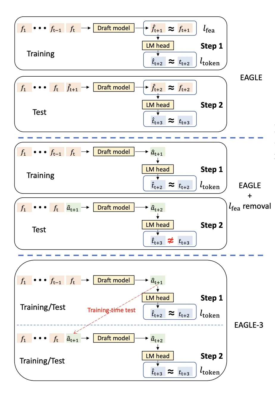 Training-time test simulates multi-step generation during training by feeding the draft head's predictions back as inputs
Here's how it works with a training example "How can I":
Native training step (predicting the first token ahead):
- Input: Perfect features from target model for ["How", "can"]
- Draft head predicts: "I"
- Target: Ground truth is "I"
- Loss: KL divergence between draft prediction and target model's distribution
Simulated step 1 (predicting the second token ahead):
- Input: Perfect features for ["How", "can"] + draft head's own prediction "I"
- Draft head predicts: "help"
- Target: Ground truth is "help"
- Loss: KL divergence between draft prediction and target model's distribution
Simulated step 2 (predicting the third token ahead):
- Input: Perfect features for ["How", "can"] + draft predictions ["I", "help"]
- Draft head predicts: "you"
- Target: Ground truth is "you"
- Loss: KL divergence
The draft head trains on all these scenarios within each batch. It learns to make good predictions given perfect inputs AND to make robust predictions given its own potentially imperfect outputs. This mixed setup better matches what happens during inference, where the draft head must condition on its own previous predictions.
Handling tree-like attention patterns
The training process requires custom attention masks. The original training data "How can I" has a standard sequential dependency (each token sees all previous tokens). But the predicted tokens "help", "you", etc. have tree-like dependencies because they branch from different prediction steps.
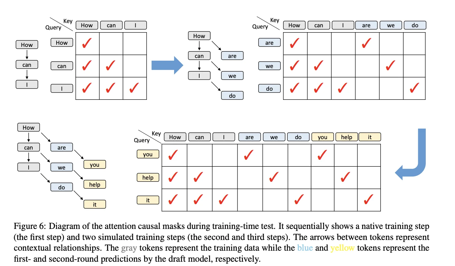 Custom attention masks during training-time test: gray tokens are training data, blue and yellow tokens are first- and second-round predictions from the draft head
EAGLE-3 handles this by computing attention scores only for relevant positions using vector dot products instead of full matrix multiplication. This avoids wasted computation on zero-masked positions and significantly reduces the overhead compared to a dense matrix-multiplication implementation.
Why this works
This training regime allows EAGLE-3 to maintain a high acceptance rate even for later predicted tokens, while methods trained only on "perfect" inputs show a clear decline as the number of self-predicted inputs grows. As shown in Figure 7 of the paper, EAGLE-3's acceptance rate stays almost flat across positions, whereas EAGLE's acceptance rate drops significantly. The draft head becomes robust to its own errors and learns to recover from mistakes, just like it must do during actual inference.
Scaling Behavior with Training Data
EAGLE-3 discovers a scaling law for speculative decoding: increasing training data leads to proportional improvements in speedup. This scaling behavior was not observed in the original EAGLE architecture.
The paper demonstrates this by training on ShareGPT (68K samples) and UltraChat-200K (464K samples), for a total of approximately 532K training examples. With roughly 8x more training data and architectural improvements, EAGLE-3 achieves about a 1.4x latency improvement over EAGLE-2 at batch size 1.
Why EAGLE-3 scales better: The feature prediction constraint in EAGLE-1 and EAGLE-2 limited the draft model's expressiveness. The draft model had to match the target model's internal features, not just predict the right tokens. Removing this constraint gives EAGLE-3 complete flexibility in what it learns from data. Combined with multi-layer feature fusion, this lets the draft model extract more useful patterns as training data increases.
Performance Characteristics
EAGLE-3 achieves speedups between 3.0x and 6.5x across different models and tasks, with an average acceptance length (τ) of 4.05 to 7.5 tokens per draft-verify cycle. On MT-bench with LLaMA-3.1-8B, EAGLE-3 reaches 4.40x speedup with τ=6.13, and 4.48x on GSM8K with τ=6.23.
In production environments using SGLang on a single H100 GPU, EAGLE-3 provides 1.81x throughput improvement at batch size 2 and maintains 1.38x improvement at batch size 64, while EAGLE-2 actually decreases throughput to 0.93x at batch size 24.
Memory overhead is minimal: the draft head adds approximately 0.25B parameters for an 8B model and 1B parameters for a 70B model. These speedups make EAGLE-3 one of the fastest LLM inference methods available without requiring specialized hardware. The method works across different model architectures (LLaMA, Qwen, DeepSeek) and tasks without modification, requiring no special hardware or kernel modifications.
When to Use EAGLE-3
EAGLE-3 is most effective in specific deployment scenarios. Understanding when to use it helps maximize the return on your training investment.
Ideal Use Cases:
-
Production serving at small-to-medium batch sizes: EAGLE-3 delivers the strongest speedups when batch sizes are small. Our benchmarks show 2.3x speedup at batch size 4 for Llama-3.1-8B. This is perfect for interactive applications, chatbots, and API endpoints where latency matters.
-
Latency-sensitive applications: When response time is critical (real-time chat, code completion, interactive assistants), EAGLE-3's 2-6x speedup directly improves user experience.
-
Cost optimization at scale: Faster inference means fewer GPU hours. For deployments serving millions of requests, a 2-4x speedup can cut infrastructure costs in half while maintaining identical output quality.
-
Larger models: The benefits scale favorably with model size. Larger models see higher speedups because draft head overhead becomes negligible while memory bandwidth savings increase. EAGLE paper shows consistent speedups across 7B to 70B models.
When NOT to use EAGLE-3:
-
Very large batch sizes: Our benchmarks show speedups drop significantly at higher batch sizes (e.g., roughly break-even at batch size 32). At these sizes, the target model becomes compute-bound rather than memory-bound, reducing speculation benefits.
-
Memory-constrained environments: While the draft head adds minimal overhead (~1.4% for 70B models), it still requires additional GPU memory. If you're already at capacity, the draft head may not fit.
-
One-off inference tasks: The training investment (multi-GPU setup, 1-2 days) only makes sense for production workloads where you'll use the draft head repeatedly.
-
Extremely high system load: Under heavy request rates with large batches, loading both draft and target models can reduce space for batch processing and potentially hurt throughput.
Practical Guidelines:
Based on our benchmark results, EAGLE-3 works best when:
- Batch sizes are small to medium (stronger benefits at lower batch sizes)
- You're deploying to production for extended periods
- Response latency directly impacts user experience or operational costs
- You have the resources for initial training (multi-GPU setup, ~532K training samples)
Training Your Own EAGLE-3 Model
Understanding the architecture is one thing, but training your own EAGLE-3 draft model is where theory becomes practice. This section walks through the complete process: setting up GPU infrastructure, preparing training data, running the training loop, and deploying for inference with SGLang.
We'll use SpecForge, the official training framework from the SGLang team. SpecForge was built specifically to make EAGLE-3 training accessible - it handles the complex attention masks, training-time test logic, and SGLang integration so you can focus on your data and model configuration.
Setting Up Your GPU Instance
Training EAGLE-3 requires GPU infrastructure. For this tutorial, we'll deploy on E2E Networks, which provides H100 and A100 instances optimized for LLM training.
Creating Your Instance
-
Log in to your E2E Networks account and navigate to the Instances (Nodes) section under Products in the left sidebar. Click the CREATE INSTANCE button.
-
You'll be asked to Choose Image. Select the PyTorch image under the Pre-built tab. This image comes pre-installed with NVIDIA drivers, CUDA, PyTorch, and other essentials, saving you setup time.
Next, choose a Plan. EAGLE-3 training works in two modes: online (where the target model runs as a server during training) and offline (where hidden states are pre-computed). This affects your GPU requirements:
Online training (recommended for getting started):
- For an 8B model like Llama-3.1-8B, you can train on a single 40GB GPU, but multi-GPU setups significantly improve throughput
- 4× A100 40GB or 4× H100 80GB: Comfortable configuration for 8B-13B models using tensor parallelism
- 8× A100 40GB or 4× H100 80GB: Good for 70B-class models or higher batch sizes
Offline training (more efficient, requires pre-computation):
- Can work with as few as 1 GPU since only the draft model loads during training
- The trade-off is storage (see below)
Choose your Instance Pricing. For cost savings, select the Spot plan if you're running experiments where interruptions are acceptable. For production training runs that can't afford interruption, stick with On-Demand or Reserved instances.
Configure Storage. Requirements vary dramatically by training mode:
- Online training: Allocate at least 200GB for model checkpoints and datasets
- Offline training: You'll need significantly more, potentially 2-5 TB, to store pre-computed hidden states for large datasets like UltraChat + ShareGPT
Add your SSH key for secure access, and configure any necessary Security Group settings to allow SSH (port 22) and any custom ports for monitoring tools.
Click Launch Instance.
Connecting to Your Instance
Once your instance status shows "Running", you can connect to it.
You have two main options:
- SSH: Use the provided SSH command in your local terminal or configure your favorite IDE (like VS Code with the Remote - SSH extension) to connect directly to the instance's IP address. This is the preferred method for training workflows.
ssh -i /path/to/your/key.pem ubuntu@<instance-ip>- Jupyter Lab: Click the Jupyter link in the instance details page to open a Jupyter Lab interface in your browser. This works well for interactive exploration and data preparation.
Installing SpecForge and Dependencies
Once connected to your instance, set up the training environment. The PyTorch image already has CUDA and PyTorch installed, but you need to add SpecForge and its dependencies.
First, create a virtual environment. SpecForge recommends Python 3.11:
# Install uv if not already available
curl -LsSf https://astral.sh/uv/install.sh | sh
source $HOME/.local/bin/env

# Create virtual environment
uv venv --python 3.11
source .venv/bin/activate
Clone the SpecForge repository and install:
git clone https://github.com/sgl-project/SpecForge.git
cd SpecForge
uv pip install -v .
This installs SpecForge along with SGLang, transformers, datasets, and all required dependencies.
Preparing Training Data
EAGLE-3 training requires conversation data in a specific format. The quality of your training data directly impacts the draft model's acceptance rate during inference. This section covers the data format requirements, how to use pre-existing datasets, and why regenerating data with your target model matters.
Why Regenerate Training Data?
Most public conversation datasets like ShareGPT or UltraChat weren't generated by your specific target model. These datasets contain responses from GPT-3.5, GPT-4, or other models. When you train an EAGLE-3 draft head using data from a different model, the draft head learns to mimic that other model's distribution rather than your target model's distribution.
This misalignment reduces acceptance rates during inference. The draft head predicts tokens it learned from GPT-4, but your target model (say, Llama-3.1-8B) would have generated different tokens. The target model rejects more draft tokens, reducing speedup.
The solution: Regenerate your training data using the target model itself. Take the user prompts from public datasets, feed them through your target model, and use those responses for training. This ensures the draft head learns to predict exactly what your target model would generate.
SpecForge provides scripts to automate this process. You can regenerate data from scratch or use pre-regenerated datasets shared by the community.
Required Data Format
SpecForge expects training data in JSONL format with this schema:
{
    "id": "unique-conversation-id",
    "conversations": [
        {
            "role": "system",
            "content": "You are a helpful assistant."
        },
        {
            "role": "user",
            "content": "What is speculative decoding?"
        },
        {
            "role": "assistant",
            "content": "Speculative decoding is a technique..."
        },
        {
            "role": "user",
            "content": "How does it work?"
        },
        {
            "role": "assistant",
            "content": "It works by predicting multiple tokens..."
        }
    ]
}
Each line in the JSONL file is one conversation. The conversations array contains the full dialogue with alternating user and assistant messages. The system message is optional but recommended if your target model was trained with a system prompt.
Key requirements:
- Each conversation needs a unique
id - Roles are typically
"user"and"assistant"in the conversation format. If your model needs a system prompt, you can include it via the pre-formatted text format that uses the chat template - Content should be the actual message text
- Conversations generally alternate between user and assistant
Using Pre-Existing Datasets
SpecForge provides scripts to download and convert popular datasets. The two main datasets used for EAGLE-3 training are:
ShareGPT (~68K samples): Multi-turn conversations covering diverse topics. These are real ChatGPT conversations shared by users.
UltraChat-200K (~464K samples): Synthetic conversations generated to cover various instruction-following scenarios.
Download and convert these datasets:
cd SpecForge

# Prepare ShareGPT dataset
python scripts/prepare_data.py --dataset sharegpt --output-path ./data

# Prepare UltraChat dataset
python scripts/prepare_data.py --dataset ultrachat --output-path ./data
The --output-path specifies where to save the processed JSONL files. If you omit this flag, files save to cache/dataset/<dataset_name> by default.
You can also limit the number of samples:
# Process only 50,000 samples from ShareGPT
python scripts/prepare_data.py --dataset sharegpt --sample-size 50000 --output-path ./data
After processing, you'll have sharegpt.jsonl and ultrachat.jsonl files ready for training or regeneration.
Regenerating Data with Your Target Model
Once you have the base datasets, regenerate them using your target model. This step is crucial for maximum performance. SpecForge provides the regenerate_train_data.py script that handles this automatically.
The script launches an SGLang server with your target model, feeds it all the user prompts from your dataset, generates new responses, and saves them in the same JSONL format.
Here's how to regenerate the ShareGPT dataset with Llama-3.1-8B-Instruct:
python scripts/regenerate_train_data.py \
    --model meta-llama/Llama-3.1-8B-Instruct \
    --input-file-path ./data/sharegpt.jsonl \
    --output-file-path ./data/sharegpt_llama31_8b.jsonl \
    --batch-size 128 \
    --tp-size 4 \
    --num-samples 50000 \
    --port 30000 \
    --temperature 0 \
    --mem-fraction-static 0.85 \
    --auto-launch-server
Parameter breakdown:
--model: HuggingFace model path or repo name for your target model--input-file-path: Your base dataset in JSONL format--output-file-path: Where to save the regenerated dataset--batch-size: Number of requests to process in parallel (adjust based on GPU memory)--tp-size: Tensor parallelism size (number of GPUs to use)--num-samples: How many conversations to regenerate (omit to process all)--temperature: Sampling temperature (0 = greedy, recommended for training data)--auto-launch-server: Automatically launch SGLang server before regeneration
The regeneration process extracts user messages from each conversation, sends them through your target model, and replaces the assistant responses with the target model's actual outputs. This typically takes several hours depending on dataset size and GPU count.
Now you have training data that closely matches your target model's distribution.
Using pre-regenerated datasets: There are pre-regenerated community datasets on HuggingFace. For Llama-3.1-8B-Instruct, you can download zhuyksir/Ultrachat-Sharegpt-Llama3.1-8B instead of regenerating from scratch.
Preparing Your Own Custom Dataset
If you have your own conversation data, SpecForge supports both standard conversation format (with separate role and content fields) and pre-formatted text (where conversations are already templated). The conversation format follows the same JSONL schema shown earlier with id and conversations fields.
For detailed instructions on preparing custom datasets, including pre-formatted text format and combining multiple datasets, see the SpecForge Data Preparation documentation.
Training the EAGLE-3 Draft Head
With your data prepared, you're ready to train the draft head. SpecForge provides an online training script that handles the entire training loop: launching the target model server, building the dataset cache, running distributed training, and saving checkpoints. This section walks through the complete training process.
Understanding Online vs Offline Training
SpecForge supports two training modes:
Online training: The target model runs as an SGLang server during training. When the draft head needs target model features, it queries the server in real-time. This is simpler to set up and works well for most cases.
Offline training: You pre-generate all target model hidden states and save them to disk. Training reads from these saved states instead of querying a server. This is faster but requires significantly more disk space (potentially several terabytes for large datasets).
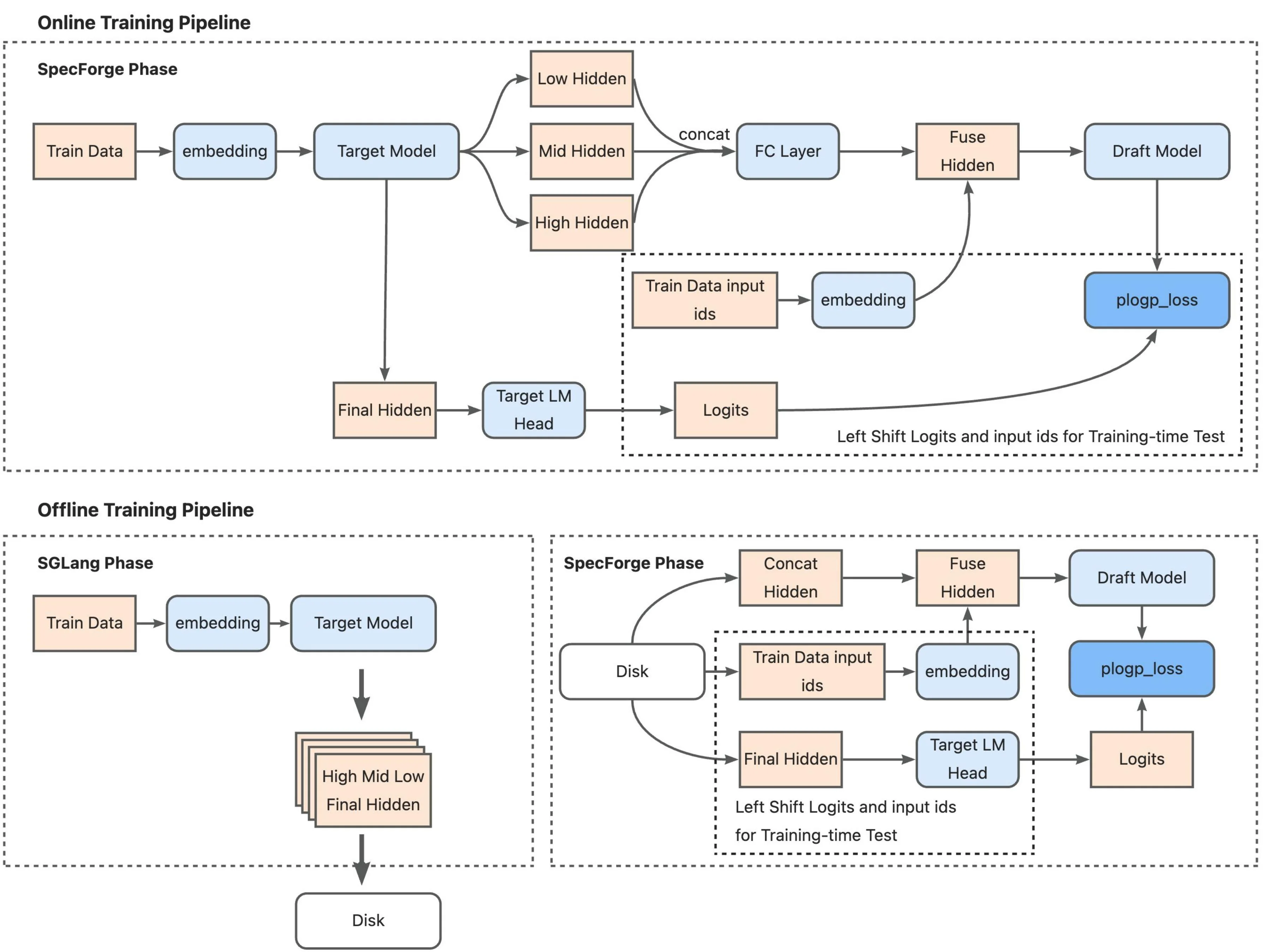 Training pipeline comparison: Online mode (top) runs the target model as an SGLang server that processes training data in real-time, extracts multi-layer features, and feeds them to the draft model for training. Offline mode (bottom) pre-computes all hidden states during an SGLang phase and stores them to disk, then loads these cached features during the SpecForge training phase, eliminating the need for a live target model server. (Source: LMSYS SpecForge Blog)
For this tutorial, we'll use online training since it's more accessible and doesn't require pre-computing hidden states.
Building the Dataset Cache
Before training, you need to preprocess your data and build a cache. This step:
- Tokenizes all conversations using the target model's tokenizer
- Applies the chat template to format system/user/assistant messages
- Generates loss masks (only assistant tokens contribute to loss, user/system tokens are masked)
- Builds a vocabulary mapping between the target model's full vocabulary and the draft model's reduced vocabulary
- Caches everything to disk for fast loading during training
Run the cache building script:
python scripts/build_eagle3_dataset_cache.py \
    --target-model-path meta-llama/Llama-3.1-8B-Instruct \
    --draft-model-config ./configs/llama3-8B-eagle3.json \
    --train-data-path ./data/merged_train.jsonl \
    --cache-dir ./cache \
    --chat-template llama3 \
    --max-length 2048 \
    --view-train-data 1
Key parameters:
--target-model-path: Your target model (must match what you'll use for training)--draft-model-config: JSON config file defining draft head architecture--train-data-path: Your training data in JSONL format--chat-template: Chat template name (llama3, qwen, chatml, etc.)--max-length: Maximum sequence length for training--view-train-data: Indices of samples to visualize (optional, useful for debugging)
The --view-train-data flag is helpful for verification. It displays training samples with color coding: green text shows tokens where the loss mask is 1 (assistant responses that contribute to training), red text shows tokens where the loss mask is 0 (user inputs and system prompts that are masked out).
The cache building process creates files in your --cache-dir directory. This only needs to run once per dataset - subsequent training runs reuse the cached data.
The Draft Model Configuration
The draft head architecture is defined in a JSON config file. For Llama-3.1-8B, the config looks like this:
{
  "model_type": "llama",
  "hidden_size": 4096,
  "num_hidden_layers": 1,
  "num_attention_heads": 32,
  "num_key_value_heads": 8,
  "intermediate_size": 14336,
  "hidden_act": "silu",
  "vocab_size": 128256,
  "draft_vocab_size": 32000
}
Important fields:
num_hidden_layers: 1: The draft head is just one transformer decoder layerhidden_size: 4096: Must match the target model's hidden dimensionvocab_size: 128256: Target model's full vocabulary sizedraft_vocab_size: 32000: Reduced vocabulary for the draft model (top-k most frequent tokens)
The draft head uses a reduced vocabulary to save memory and computation. During training, SpecForge builds a mapping from the target model's 128K vocabulary to the draft model's 32K vocabulary, keeping only the most frequently used tokens.
Running the Training
Launch training using PyTorch's distributed launcher:
export NUM_GPUS=4

torchrun \
    --standalone \
    --nproc_per_node $NUM_GPUS \
    scripts/train_eagle3_sgl_online.py \
    --target-model-path meta-llama/Llama-3.1-8B-Instruct \
    --model-path meta-llama/Llama-3.1-8B-Instruct \
    --draft-model-config ./configs/llama3-8B-eagle3.json \
    --train-data-path ./data/merged_train.jsonl \
    --tp-size $NUM_GPUS \
    --output-dir ./outputs \
    --num-epochs 10 \
    --batch-size 1 \
    --learning-rate 5e-5 \
    --draft-attention-backend flex_attention \
    --max-length 2048 \
    --chat-template llama3 \
    --cache-dir ./cache \
    --mem-frac 0.4 \
    --total-steps 800000 \
    --warmup-ratio 0.015 \
    --save-interval 10000 \
    --log-interval 100 \
    --report-to wandb \
    --wandb-project eagle3-llama31-8b \
    --wandb-name training-run-1
Critical parameters:
--nproc_per_node: Number of GPUs to use (must match--tp-size)--target-model-path: Target model for generating features and serving during training--draft-model-config: Draft head architecture config--train-data-path: Training data (same file used for cache building)--tp-size: Tensor parallelism size (distribute target model across this many GPUs)--num-epochs: Number of complete passes through the training data--learning-rate: Learning rate (5e-5 recommended for Llama models)--total-steps: Total training steps (800K recommended for publication-quality results)--warmup-ratio: Learning rate warmup ratio (1.5% of total steps)--draft-attention-backend: Useflex_attentionfor efficient tree attention (requires PyTorch 2.5+)--mem-frac: GPU memory fraction for target model server (0.4 leaves room for draft model training)
Training hyperparameters:
--batch-size 1: Batch size per GPU (the actual global batch size is controlled by gradient accumulation)--draft-global-batch-size 16: Global batch size for draft head training (default if not specified)--max-grad-norm 0.5: Gradient clipping threshold--ttt-length 7: Training-time test length (how many tokens ahead to predict during training)
Checkpointing and logging:
--output-dir: Where to save model checkpoints--save-interval 10000: Save checkpoint every N steps--log-interval 100: Log metrics every N steps--report-to wandb: Track training with Weights & Biases (alternatives: tensorboard, swanlab, mlflow)
What Happens Inside the Training Loop
When you launch training, SpecForge executes the following steps:
Initialization:
- Launches an SGLang server with the target model distributed across GPUs using tensor parallelism
- Loads the draft head model and initializes it with random weights
- Loads the dataset cache built in the previous step
- Sets up FSDP (Fully Sharded Data Parallel) for efficient distributed training of the draft head
- Initializes the optimizer (AdamW with BF16 mixed precision) and learning rate scheduler
For each training batch:
- Load tokenized conversations from the dataset cache
- Generate target model features: Query the SGLang server to get hidden states from multiple layers (low, middle, high) of the target model for the current batch
- Fuse multi-layer features: Concatenate features from the three layers and compress them through a learned projection layer
- Draft head forward pass with training-time test:
- Native prediction (step 0): Use target model features to predict the next token
- Simulated prediction (steps 1-6): Feed the draft head's own predictions back as input to simulate multi-step generation during inference
- Generate predictions for all positions up to
--ttt-length(default 7 steps ahead)
- Compute custom tree attention masks: Create sparse attention patterns that reflect the tree-like dependencies during multi-step prediction
- Calculate KL divergence loss: Compare draft head predictions against target model probability distributions at each position
- Backpropagate and update: Compute gradients, clip them, and update draft head weights
- Log metrics: Track loss, learning rate, throughput, and other training statistics
Monitoring Training Progress
Training produces several metrics to monitor:
- Loss: KL divergence between draft and target distributions (should decrease over time)
- Learning rate: Follows warmup schedule then decays
- Throughput: Samples processed per second
- GPU memory: Target model server + draft head training
- Gradient norms: Should stay below
max_grad_normthreshold
Training Configuration from SpecForge Examples
The SpecForge repository provides reference training configurations that align with the official EAGLE paper. For Llama-3.1-8B training:
Verified training parameters:
- Total training steps: 800,000 steps (from SpecForge example scripts, aligns with EAGLE official repo config)
- Number of epochs: 10 epochs over the training data
- GPUs: 4 GPUs with tensor parallelism
- Batch size: 1 per GPU
- Learning rate: 5e-5 with 1.5% warmup ratio
- Memory fraction: 0.4 for target model server (leaves room for draft head training)
Training data scale: The paper uses ShareGPT and UltraChat datasets. The example scripts reference pre-regenerated datasets like zhuyksir/Ultrachat-Sharegpt-Llama3.1-8B which combine both datasets regenerated with Llama-3.1-8B.
Hardware requirements: Training requires multi-GPU setup (4-8 GPUs recommended). The target model runs as an SGLang server consuming a portion of GPU memory (controlled by --mem-frac), while the draft head training uses the remaining memory with FSDP for distributed training.
Time and cost: Training time and cost will depend on your specific hardware, dataset size, and cloud provider pricing. Monitor your first few hundred steps to estimate throughput (samples/second), then extrapolate for 800K total steps.
Once training completes, your draft head checkpoints are ready for inference deployment with SGLang.
Benchmark Results: Real-World Performance
Training is one thing. What matters is whether the draft head actually speeds up inference in practice. To find out, we followed the training process outlined above using the SpecForge reference configuration: 4 GPUs, online training mode, and the combined ShareGPT + UltraChat dataset regenerated with Llama-3.1-8B. After training completed, we ran the draft head through inference benchmarks to measure real-world speedups.
Setup
We tested the trained draft head using SGLang on a single A100 GPU across four different tasks and three batch sizes. We used SpecForge's official benchmarking script which automates the entire process:
- Target model: meta-llama/Llama-3.1-8B-Instruct
- Draft model: Our trained EAGLE-3 draft head (following the training process described above)
- Benchmarks: MT-bench (80 samples), GSM8K (200 samples), HumanEval (200 samples), MATH500 (200 samples)
- Batch sizes tested: 4, 8, and 32
- Draft configuration: 5 speculative steps, topk=8, 32 verification tokens
The benchmark compared vanilla autoregressive generation (no speculation) against EAGLE-3 accelerated generation, measuring throughput in tokens per second.
What We Found
The speedups varied significantly by batch size:
| Batch Size | Benchmark | Vanilla (tok/s) | EAGLE-3 (tok/s) | Speedup | Acc Length |
|---|---|---|---|---|---|
| 4 | GSM8K | 560 | 1,215 | 2.17x | 4.68 |
| HumanEval | 578 | 1,457 | 2.52x | 5.09 | |
| MATH500 | 577 | 1,283 | 2.22x | 4.44 | |
| MT-bench | 562 | 1,292 | 2.30x | 4.58 | |
| Average | 569 | 1,312 | 2.30x | 4.70 | |
| 8 | GSM8K | 1,040 | 1,870 | 1.80x | 4.67 |
| HumanEval | 1,094 | 2,328 | 2.13x | 5.09 | |
| MATH500 | 1,091 | 2,072 | 1.90x | 4.41 | |
| MT-bench | 1,052 | 2,138 | 2.03x | 4.60 | |
| Average | 1,069 | 2,102 | 1.97x | 4.69 | |
| 32 | GSM8K | 2,979 | 2,649 | 0.89x | 4.67 |
| HumanEval | 3,445 | 3,475 | 1.01x | 5.09 | |
| MATH500 | 3,501 | 3,167 | 0.90x | 4.41 | |
| MT-bench | 3,084 | 3,454 | 1.12x | 4.63 | |
| Average | 3,252 | 3,186 | 0.98x | 4.70 |
What This Means
Batch size has a huge impact: At batch size 4, EAGLE-3 delivers 2.3x speedup, but this drops to roughly break-even at batch size 32. This happens because larger batch sizes increase GPU utilization for the target model. More of the GPU's compute is already occupied by the target model at high batch sizes, so the extra draft work has less "free" bandwidth to use. The target model becomes compute-bound rather than memory-bound, reducing the benefits of speculation.
Different tasks, different speedups: HumanEval consistently shows the best speedups (2.52x at batch 4), while GSM8K and MATH500 are slightly lower. This matches what the EAGLE-3 paper found: code generation has many fixed templates and predictable patterns, making it easier for the draft head to predict correctly. Mathematical reasoning is less predictable.
Draft head quality stays solid: Across all batch sizes, the average acceptance length remains around 4.5-5.0 tokens per draft-verify cycle. This means the draft head quality doesn't degrade with batch size. The reduced speedup at high batches is purely because the baseline target model throughput increases, not because the draft head gets worse.
How This Compares to the Paper
These numbers are from our internal benchmarks on Llama-3.1-8B using SGLang + A100. The original EAGLE-3 paper reports speedups between 3.0x and 6.5x across multiple models using a slightly different evaluation stack. Our 2.3x at batch size 4 sits well within that range for an 8B model.
Why Larger Models Often See Better Speedups
Our results are for Llama-3.1-8B, a relatively small model. Larger models (70B, 100B, 200B parameters) often see equal or better speedups for two reasons:
Memory bandwidth becomes the bottleneck: Larger models spend more time moving parameters from GPU memory to compute units. An 8B model's 16GB of parameters can stay in cache more easily than a 200B model's 400GB. EAGLE-3 reduces the number of target model forward passes, so the memory traffic savings matter more as models get bigger.
Draft head overhead becomes negligible: The draft head is tiny compared to the backbone. It adds roughly 0.2-0.3B parameters for an 8B model and around 1B parameters for a 70B model. That's a few percent or less of the base model. For 200B-class models, it's under 1% overhead. The relative cost of running the draft head decreases as the target model grows, while the benefit (avoiding full forward passes) stays constant.
The paper reports speedups around 4.0-4.8x for LLaMA-3.3-70B across different tasks. In practice, if you match the paper's training and decoding setup, 70B-class models often land in the 4-6x speedup range at low batch sizes.
EAGLE-3 vs Other Speculative Decoding Methods
Understanding how EAGLE-3 compares to alternative speculative decoding approaches helps you choose the right optimization strategy for your use case.
| Method | Draft Approach | Speedup Range | Training Required | Memory Overhead | Key Advantage | Key Limitation |
|---|---|---|---|---|---|---|
| EAGLE-3 | Lightweight draft head with multi-layer fusion and training-time test | 3.0-6.5x | Yes (~532K samples: ShareGPT + UltraChat) | <5% of base model | Best scaling with training data, highest acceptance rates (70-80%) | Requires more training data for optimal performance |
| EAGLE-2 | Dynamic draft head with context-aware tree structure | 3.05-4.26x (20-40% over EAGLE-1) | No (reuses EAGLE-1 head) | ~1.4% (same as EAGLE-1) | Improved performance without retraining | Inherits EAGLE-1's limited data scaling |
| EAGLE (Original) | Single-layer draft head reusing top-layer features | 2.2-3.8x | Yes (~68K ShareGPT samples, 1-2 days) | ~1.4% (0.99B params for 70B model) | Simple and effective, lossless acceleration | Limited improvement from additional training data |
| Medusa | Multiple prediction heads (3-5 heads) on top of hidden states | 2.2-2.8x (Medusa-1: 2.2x, Medusa-2: 2.4-2.8x) | Yes (can be done on single GPU) | Low (single-layer heads, reuses LM head weights) | Simple architecture, self-distillation option | Lower speedups compared to EAGLE-family methods |
| SpecInfer | Multiple small speculative models (100-1000× smaller) | 1.5-3.5x | No (uses existing smaller models) | <1% per small model | No training needed, uses pre-existing models | Requires compatible smaller models from same family |
When to choose EAGLE-3:
- Maximum performance required (production serving at small-to-medium batch sizes)
- Access to training resources and large datasets (ShareGPT + UltraChat: ~532K samples)
- Working with larger models where benefits are especially strong (though effective across 7B-70B+ range)
- Need consistent performance across multiple tasks without task-specific tuning
When to choose other methods:
- EAGLE-2: Already have EAGLE-1 head trained and want 20-40% boost without retraining
- EAGLE (Original): Budget-constrained training, limited data (~68K samples sufficient)
- Medusa: Single GPU training, self-distillation when no training data available, simplest architecture
- SpecInfer: Zero training budget, working with established model families that have smaller siblings (e.g., OPT, LLaMA)
Important Note: All speculative decoding methods see diminishing benefits at very high batch sizes where the target model becomes compute-bound rather than memory-bound.
Frequently Asked Questions
How much faster is EAGLE-3 than standard inference?
EAGLE-3 achieves speedups between 2-6x depending on the model size and batch configuration. For Llama-3.1-8B at batch size 4, our benchmarks show 2.3x speedup. Larger models (70B+) typically see higher speedups in the 4-6x range because the draft head overhead becomes negligible while memory bandwidth savings increase.
Does EAGLE-3 work with all language models?
EAGLE-3 works with any decoder-only transformer model. The method has been successfully tested with LLaMA, Qwen, and DeepSeek architectures. You need to train a draft head specifically for your target model using the model's own generated data, but once trained, the same draft head works across different tasks (code generation, math reasoning, instruction following) without task-specific fine-tuning.
What are the implementation costs of EAGLE-3?
The upfront implementation cost depends on your model size and the amount of training data you use. Smaller models with limited data require less compute resources and time, while larger models with extensive datasets need more powerful multi-GPU infrastructure and longer training runs. However, this is a one-time cost. Once the draft head is trained, you can use it infinitely for all your inference workloads without retraining. The long-term benefit is significant: faster inference translates to lower operational costs, better user experience, and reduced infrastructure spend at scale.
When should I use EAGLE-3 vs other optimization methods?
Use EAGLE-3 when you're running inference at small to medium batch sizes (1-16) where latency matters more than raw throughput. It's ideal for production serving, interactive applications, and cost optimization scenarios. EAGLE-3 works best alongside other optimizations like quantization and efficient attention. Avoid it for very large batch sizes (32+) where the target model becomes compute-bound and speculation benefits diminish.
Conclusion
EAGLE-3 makes LLM inference 2-6x faster without changing the model or sacrificing output quality. Instead of generating one token at a time, you train a lightweight draft head that predicts multiple tokens ahead, which the target model verifies in parallel. The draft head adds under 5% parameters, reuses the target model's internal features, and works across different tasks without fine-tuning.
We covered the complete implementation pipeline: how EAGLE-3's architecture works (training-time test, multi-layer feature fusion, dynamic tree generation), how to set up GPU infrastructure on E2E Networks, how to prepare and regenerate training data, how to train the draft head with SpecForge, and how to benchmark the results.
Our benchmarks show 2.3x speedup on Llama-3.1-8B at batch size 4, with acceptance lengths around 4.5-5.0 tokens per verification cycle. The EAGLE-3 paper reports 4-6x speedups for 70B-class models. These speedups translate directly to cutting infrastructure costs in half while maintaining identical output quality.
For teams looking to optimize LLM inference at scale, EAGLE-3 is one of the most practical ways to reduce latency and cost. With lightweight training on a few GPUs, the draft head works immediately after training with no integration overhead. For production deployments serving millions of requests, that's a significant win.
References
-
EAGLE-3: Speculative Sampling with Cascade of Contextual Fusion for Fast Decoding : The official EAGLE-3 paper by Yuanyuan Li et al. Introduces training-time testing, multi-layer feature fusion, and demonstrates 3.0-6.5x speedups across multiple models and tasks.
-
An Introduction to Speculative Decoding for Reducing Latency in AI Inference: NVIDIA Developer Blog explaining the fundamentals of speculative decoding, draft-target verification, and the parallel generation approach.
-
SpecForge: Efficient Training Framework for EAGLE-3: LMSYS blog post introducing SpecForge, the official training framework for EAGLE-3. Covers online/offline training modes, implementation details, and integration with SGLang.
-
SpecForge Documentation: Official SpecForge documentation with detailed guides on data preparation, training configuration, and deployment with SGLang inference server.


